Estimate
1
V
7
Estimated integer ambiguities are stochastic
Lustrumboek "The 5th Element"
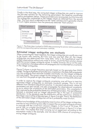
Finally in the third step, the computed integer ambiguities are used to improve
the first-step solution tor the remaining parameters, like baseline-coordinates
and/or atmospheric delays These parameters are recomputed, but this time with
the ambiguities constrained to the integer values as obtained from the second
step. This final result is referred to as the 'fixed' solution and it generally inherits
a much higher precision than the previously obtained 'float solution'.
'Float' solution
Estimate
position and
carrier
am biguities
Least squares
LAMBDA method
integer
am biguities
Integer least squares
'Fixed' solution
Estimate
position
(am big uities
fixed)
Least squares
F/gure 1: The three steps involved in GNSS doto processing for precise relative positioning
and the corresponding optimal estimation methods.
When computing the 'fixed' baseline, the integer ambiguities are usually assumed
to be known with certainty But how sure can one be? After all, the inteqer
ambiguities are determined from noisy data. Only in the hypothetical case of
Pu observaxtlons without any noise or errors, would the float solution always
yield the correct integer ambiguity values. In reality, however, this is not the case
Any uncertainty in the observations will propagate and manifest itself as uncertainty
in the integer ambiguities. 1
F'9 jreï ?LSh?WS a.niln9,e-frequency example based on the geometry-free GNSS
model. I he figure illustrates empirically how uncertainty in the data (left) propagates
into the ambiguity float estimate (middle) and finally into the integer ambiquity
estimate (rightl. The correct integer for the ambiguity is 4 in this case, but as one
can see trom the graph at right, also other integer values are frequently obtained.
In order to capture the integer ambiguity uncertainty, one will have to treat the
estimated integer ambiguities as stochastic (random) variates. This is not too
different trom standard adjustment practice. In standard adjustments, where all
parameters are real-valued, one also propagates the observational uncertainty
so as to obtain the uncertainty of the estimated parameters. This uncertainty is
then captured by the probability distribution of these parameters. The real difference
between a standard and an integer adjustment lies in the type of probability
distribution. In the standard case the distribution will be continuous, whereas in
the integer case it will be of discrete type, cf. figure 2 at right. That is, the distribution
ot the estimated integer ambiguities will be a probability mass function.
Without any knowledge of the probability mass function of the integer ambiguities,
one has no way of knowing how often to expect the computed ambiguity solution
to coincide with the correct but unknown integers. Is this 9 out of 1 0 times, 99
?ut ^'9.'ler percentage? In the example shown in figure 2 it is'less
than 45/o. I his implies that when carrying out an experiment according to the
assumption made in the example, one has about 55% chance of computinq a
wrong integer ambiguity.
104