Lustrumboek The 5th Element"
As far as the data processor concerns we are confronted with a number of
theoretical and numerical problems, most of them have not yet been fully solved
The numerical problems are caused by the huge number of observations and
unknowns to be solved for (figure 1 4), which are extremely demanding in terms
of computer power and storage requirements They require efficient algorithms
and supercomputing facilities. For instance, when using a sophisticated functional
model, which allows for instance for real, perturbed orbits, satellite maneuvers,
and data gaps, all entries of the normal matrix are non-zero Currently there is
no operational approac h for the assembly of the observation equations and the
full normal equations. The solution of normal equations itself does not pose any
problem from a mathematical point of view: iterative solvers have to be used,
e g conjugate gradient methods or multigrid techniques. A critical point could
be the number of iterations. However, since the normal matrix shows a dominant
block diagonal structure with some resonance side bands, we may exploit this to
design efficient preconditioners in order to reduce the number of iterations This
has still to be investigated.
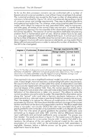
degree n
unknows
observations
Storage requirements (GB)
Design matrix
nórmal matrix
70
5037
19600
0.8
02
180
32757
129600
34.0
8.4
240
58077
230400
104.5
26.4
Figure 14: Number of observations and unknowns and storage requirements for
estimation of pofenfial oefficients from gravity gradiomefry observations. The number of
observations has been estimated using the Nyquist sampling theorem; during a real
mission the number of observations may be 10 times as large
One approach is to use a simplified functional model, for which we assume that
orbit, mission length, maximal resolution, and sampling fulfil certain requirements.
We assume that we have an uninterrupted time series of observations available
along a circular repeat orbit with a prime number has to be larger than twise the
maximal degree of the potetial field. Then, the normal equation matrix has a
block diagonal structure even when coloured noise and^or band-limited stochastic
behaviour of the observations is taken into account. This allows to solve the
normal equations very easily order by prder, We assemble the observation vector
along the "actual" orbit and take a realistic stochastic behaviour of the
measurements (e.g. coloured noise or even band-limitation) properly into account.
Then, the strategy is to reduce the influence of model errors on the gravity field
parameters by iteration. We have shown that this method converges to the proper
solution and that it can be done within reasonable time limits. We end an experiment
where a non-polar, non-circular GOCE-like orbit was simulated along which
gravity gradients were computed using a potential model up to degree and order
180. From this time series of gravity gradients the potential coefficients were
estimated up to degree and order 180 and the relative differences between
input coefficients and estimated coefficients were computed This proces was
then iterated The results are shown in figure 1 5. The lowest curve in the figure is
the one-step solution for a non-polar, circular orbit. It seems that after a few
iterations the influence of the non perfect functional model (in this case the
assumption of a circular orbit) on the estimated gravity field parameters is
negligible. However, before a definite answer can be given, more numerical
experiments have to be done
16